|
Introduction
One aspect of most sets of data is that the values are not all
alike; indeed, the extent to which they are unalike, or vary
among themselves, is of basic importance in statistics.
Consider the following examples:
In a
hospital where each patient's pulse rate is taken three times a
day, that of patient A is 72, 76, and 74, while that of
patient B is 72, 91, and 59. The mean pulse rate of the two
patients is the same, 74, but observe the difference in
variability. Whereas patient A's pulse rate is stable, that of
patient B fluctuates widely.
A
supermarket stocks certain 1-pound bags of mixed nuts, which on
the average contain 12 almonds per bag. If all the bags contain
anywhere from 10 to 14 almonds, the product is consistent and
satisfactory, but the situation is quite different if some of
the bags have no almonds while others have 20 or more.
Measuring variability is of special importance in statistical
inference.
Suppose, for instance, that we have a coin that is slightly bent
and we wonder whether there is still a fifty-fifty chance for
heads. What If we toss the con 100 times and get 28 heads and 72
tails? Does the shortage of heads-only 28 where we might have
expected 50-imply that the count is not "fair?" To answer such
questions we must have some idea about the magnitude of the
fluctuations, or variations, that are brought about by chance
when coins are tossed 100 times.
We
have given these three examples to show the need for measuring
the extent to which data are dispersed, or spread out; the
corresponding measures that provide this information are called
measures of variation. In Sections 1 through 3 we present the
most widely used measures of variation and some of their special
applications. Some statistical descriptions other than measures
of location and measures of variation are discussed in Section
4.5.
|
|
|
5.1 The
Range
To
introduce a simple way of measuring variability, let us refer to
the first of the three examples cited previously, where the
pulse rate of patient A varied from 72 to 76 while that of
patient B varied from 59 to 91. These extreme (smallest
and largest) values are indicative of the variability of the two
sets of data, and just about the same information is conveyed if
we take the differences between the respective extremes. So, let
us make the following definition:
The
range of 8 set of data is the difference between the largest
value and the smallest.
For
patient A the pulse rates had a range of 76 -72 = 4 and for
patient B they had a range of 91 -59 = 32, and for the waiting
times between eruptions of Old Faithful in Example 2.4, the
range was 118 -33 = 85 minutes.
Conceptually, the range is easy to understood, its calculation
is very easy, and there is a natural curiosity about the
smallest and largest values. Nevertheless, it is not a very
useful measure of variation - its main shortcoming being that it
does not tell us anything about the dispersion of the values
that fall between the two extremes.
For example, each of the following three sets of data
Set
A: 5 18 18 18 18 18 18 18 18 18
Set
B: 5 5 5 5 5 18 18 18 18 18
Set
C: 5 6 8 9 10 12 14 15 17 18
has
a range of 18 -5 = 13, but their dispersions between the first
and last values are totally different
In actual practice, the range is used mainly as a "quick and
easy" measure of variability;
for instance, in industrial quality control it is used to keep a
close check on raw materials and products on the basis of small
samples taken at regular intervals of time.
Whereas, the range covers all the values in a sample, a similar
measure of variation covers (more or less) the middle 50
percent. It is the inter quartile range: Q3 –Q1,
where Q1 and Q3 may be defined as before.
For instance, for the twelve temperature readings in Example
3.16 we might use 88 -76 = 12 and for the grouped data in
Example 3.24 we might use 87.58 -69.71 = 17.87. Some
statisticians also use the semi-inter quartile range ,
which is sometimes referred to as the quartile deviation. ,
which is sometimes referred to as the quartile deviation. |
|
|
5.2 The
Variance and the Standard Deviation
To
define the standard deviation, by far the most generally useful
measure of variation. Let us observe that the dispersion of a
set of data is small if the values are closely bunched about
their mean, and that it is large if the values are scattered
widely about their mean. Therefore, it would seem reasonable to
measure the variation of a set of data in terms of the amounts
by which the values deviate from their mean. If a set of numbers
x1,
x2, x3, … and xn
constitutes a sample with the mean
 ,
then the differences ,
then the differences

are called the deviation from the mean, and we might use their average (that is, their mean) as a
measure of the variability of the sample. Unfortunately,
this will not do. Unless the x’s are all equal, some of the
deviations from the mean will be positive, some will be
negative, the sum of deviations from the mean,
 ,
and hence also their mean, is always equal to zero. ,
and hence also their mean, is always equal to zero.
Since we are really interested in the magnitude of the
deviations, and not in whether they are positive or negative, we
might simply ignore the signs and define a measure of variation
in terms of the absolute values of the deviations from the mean.
Indeed, if we add the deviations from the mean as if they
were all positive or zero and divide by n, we obtain the
statistical measure that is called the mean deviation. This
measure has intuitive appeal, but because the absolute values if
leads to serious theoretical difficulties in problems of
inference, and it is rarely used.
An alternative approach is to work with the squares of the
deviations from the mean, as this will also eliminate the effect
of signs. Squares of real numbers cannot be negative; in fact,
squares of the deviations from a mean are all positive unless a
value happens to coincide with the mean. Then, if we average the
squared deviation from the mean and take the square root of the
result (to compensate for the fact that the deviations were
squared), we get

and
this is how, traditionally, the standard deviation used to be
defined. Expressing literally what we have done here
mathematically, it is also called the root-mean-square
deviation.
Nowadays, it is customary to modify this formula by dividing
the sum of the squared deviations from the mean by n-1 instead
of n. Following this practice, which will be explained
later, let us define the sample standard deviation, denoted by
s, as
|
Sample Standard Deviation |
 |
And
its square, the sample variance, as
|
Sample Variance |
 |
These formulas for the standard deviation and the variance apply
to samples, but if we substitute
 for
and
N for n, we obtain analogous formulas for the standard deviation
and the variance of a population. It is customary to denote the
population standard deviation by for
and
N for n, we obtain analogous formulas for the standard deviation
and the variance of a population. It is customary to denote the
population standard deviation by
 (sigma,
the Greek letter for lower case) when dividing by N, and by S
when dividing by N-1. Thus, for
we
write (sigma,
the Greek letter for lower case) when dividing by N, and by S
when dividing by N-1. Thus, for
we
write
|
Population Standard Deviation |
 |
and
the population variance is
 . .
Ordinarily, the purpose of calculating a sample statistics
(such as the mean, the standard deviation, or the variance) is
to estimate the corresponding population parameter. If we
actually took many samples from a population that has the mean,
calculated the sample means,
and then averaged all these estimated of,
we should find that their average is very close to
.
However, if we calculated the variance of each sample by means
of the formula  and
then averaged all these supposed estimates of
.
Theoretically, it can be shown that we can compensate for this
by dividing by n-1 instead of n in the formula for s2.
Estimators, having the desirable property that their values
will, on the average, equal the quantity they are supposed to
estimate are said to be unbiased; otherwise, they are said to be
biased. So, we say that
is
an unbiased estimator of the population mean
and
that s2 is an unbiased estimator of the population
variance.
It does not follow from this that s is also an unbiased
estimator of and
then averaged all these supposed estimates of
.
Theoretically, it can be shown that we can compensate for this
by dividing by n-1 instead of n in the formula for s2.
Estimators, having the desirable property that their values
will, on the average, equal the quantity they are supposed to
estimate are said to be unbiased; otherwise, they are said to be
biased. So, we say that
is
an unbiased estimator of the population mean
and
that s2 is an unbiased estimator of the population
variance.
It does not follow from this that s is also an unbiased
estimator of  ,
but when n is large the bias is small and can usually be
ignored. ,
but when n is large the bias is small and can usually be
ignored.
In
calculating the sample standard deviation using the formula by
which it is defined, we must (1) find
,
(2) determine the n deviations from the mean
 ,
(3) square these deviations, (4) add all the squared deviations,
(5) divide by n-1, and (6) take the square root of the result
arrived at in step 5. In actual practice, this formula is rarely
used – there are various shortcuts – but we shall illustrate it
here to emphasize what is really measured by a standard
deviation. ,
(3) square these deviations, (4) add all the squared deviations,
(5) divide by n-1, and (6) take the square root of the result
arrived at in step 5. In actual practice, this formula is rarely
used – there are various shortcuts – but we shall illustrate it
here to emphasize what is really measured by a standard
deviation.
Example (1)
A
bacteriologist found 8, 11, 7, 13, 10, 11, 7, and 9
microorganism of a certain kind in eight cultures. Calculate s.
Solution:
First calculating the mean, we get

and
then the work required to find
 may
be arranged as in the following table: may
be arranged as in the following table:
|
 |
|
 |
|
8
11
7
13
10
11
7
9 |
-1.5
1.5
-2.5
3.5
0.5
1.5
-2.5
-0.5 |
2.25
2.25
6.25
12.25
0.25
2.25
6.25
0.25 |
|
|
0.0 |
32.00 |
Finally, dividing 32.00 by 8 -1 = 7 and taking the square root
(using a simple handheld calculator), we get

rounded to two decimals
Note
in the preceding Table that the total for the middle column is
zero; since this must always be the case; it provides a
convenient check on the calculations.
It
was easy to calculate s in this Example because the data were
whole numbers and the mean was exact to one decimal. Otherwise,
the calculations required by the formula defining s can
be quite tedious, and, unless we can get s directly with
a statistical calculator or a computer, it helps to use the
formula
|
Computing formula for the sample standard deviation |
 |
Example (2)
Use
this computing formula to rework Example (1).
Solution:
First we calculate  and and
 ,
getting ,
getting

and


Then, substituting these totals and n = 8 into the formula for Sxx,
and n-1 = 7 and the value obtained for Sxx into the
formula for s, we get

and,
hence,  rounded
to two decimals. This agrees, as it should, with the result
obtained before. rounded
to two decimals. This agrees, as it should, with the result
obtained before.
As
should have been apparent from these two examples, the
advantage of the computing formula is that we got the result
without having to determine
and
work with the deviations from the mean. Incidentally, the
computing formula can also be used to find
with
the n in the formula for Sxx and the n -1 in the
formula for s replaced by N.
In
the introduction to this chapter we gave three examples in which
knowledge about the variability of the data was of special
importance. This is also the case when we want to compare
numbers belonging to different sets of data. To illustrate,
suppose that the final examination in a French course consists
of two parts, vocabulary and grammar, and that a certain student
scored 66 points in the vocabulary part and 80 points in the
grammar part. At first glance it would seem that the student did
much better in grammar than in vocabulary, but suppose that all
the students in the class averaged 51 points in the vocabulary
part with a standard deviation of 12, and 72 points in the
grammar part with a standard deviation of 16. Thus, we can argue
that the student's score in the vocabulary part is
 standard
deviations above the average for the class, while her score in
the grammar part is only standard
deviations above the average for the class, while her score in
the grammar part is only
 standard
deviation above the average for the class. Whereas the original
scores cannot be meaningfully compared, these new scores,
expressed in terms of standard deviations, can. Clearly, the
given student rates much higher on her command of French
vocabulary than on her knowledge of French grammar, compared to
the rest of the class. standard
deviation above the average for the class. Whereas the original
scores cannot be meaningfully compared, these new scores,
expressed in terms of standard deviations, can. Clearly, the
given student rates much higher on her command of French
vocabulary than on her knowledge of French grammar, compared to
the rest of the class.
What
we have done here consists of converting the grades into
standard units or z-scores. It general, if x is a
measurement belonging to a set of data having the mean
(or)
and the standard deviation s (or
),
then its value in standard units, denoted by z, is
|
Formula for Converting to Standard Units |
 |
Depending on whether the data constitute a sample or a
population. In these units, z tells us how many standard
deviations a value lies above or below the mean of the set of
data to which it belongs. Standard units will be used frequently
in application.
Example (3)
Mrs.
Clark belongs to an age group for which the mean weight is 112
pounds with a standard deviation of 11 pounds, and Mr. Clark,
her husband, belongs to an age group for which the mean weight
is 163 pounds with a standard deviation of 18 pounds. If Mrs.
Clark weighs 132 pounds and Mr. Clark weighs 193 pounds, which
of the two is relatively more overweight compared to his / her
age group?
Solution:
Mr.
Clark's weight is 193 -163 = 30 pounds above average while Mrs.
Clark's weight is "only" 132 -112 = 20 pounds above average, yet
in standard units we get
 for
Mr. Clark and for
Mr. Clark and  for
Mrs. Clark. for
Mrs. Clark.
Thus, relative to them age groups Mrs. Clark is somewhat more
overweight than Mr. Clark.
A
serious disadvantage of the standard deviation as a measure of
variation is that it depends on the units of measurement. For instance, the weights of certain objects may have a standard
deviation of 0.10 ounce, but this really does not tell us
whether it reflects a great deal of variation or very little
variation. If we are weighing the eggs of quails, a standard
deviation of 0.10 ounce would reflect a considerable amount of
variation, but this would not be the case if we are weighing,
say, 100-pound bags of potatoes. What we need in a situation
like this is a measure of relative variation such as the
coefficient of variation, defined by the following formula:
|
Coefficient of variation |
 |
The coefficient of variation expresses the standard deviation as
a percentage of what is being measured, at least on the average.
Example (4)
Several measurements of the diameter of a ball bearing made with
one micrometer had a mean of 2.49mm and a standard deviation of
0.012mm, and several measurements of the unstretched length of a
spring made with another micrometer had a mean of 0.75 in. with
a standard deviation of 0.002 in. Which of the two micrometers
is relatively more precise?
Solution:
Calculating the two coefficients of variation, we get

Thus, the measurements of the length of the spring are
relatively less variable, which means that the second micrometer
is more precise.
|
|
|
5.3 The Description of
Grouped Data
As
we saw in before, the grouping of data entails some loss of
information. Each item has lost its identity and we know only
how many values there are in each class or in each category.
To define the standard deviation of a distribution we shall have
to be satisfied with an approximation and, as we did in
connection with the mean, we shall treat our data as if all the
values falling into a class were equal to the corresponding
class mark. Thus, letting x1, x, ..., and
xk denote the class marks, and f1, f2,
..., and fk the corresponding class frequencies, we
approximate the actual sum of all the measurements or
observations with
Sx.f
= x1f1+ x2f2 + ….. xkfk
and the sum of their squares with

Then, we write the computing formula for the standard
deviation of grouped sample data as

Which is very similar to the corresponding computing formula for
s for ungrouped data. To obtain a corresponding computing
formula for,
we replace n by N in the formula for Sxx and n -1 by
N in the formula for s.
When
the class marks are large numbers or given to several decimals,
we can simplify things further by using the coding suggested below. When the class intervals are all equal, and
only then, we replace the class marks with consecutive
integers, preferably with 0 at or near the middle of the
distribution. Denoting the coded class marks by the letter
u, we then calculate Sxx and substitute into the
formula

This
kind of coding is illustrated by Figure 5.1, where we find that
if u varies (is increased or decreased) by 1, the corresponding
value of x varies (is increased or decreased) by the class
interval c. Thus, to change su from the u-scale to
the original scale of measurement, the x-scale, we multiply it
by c.
|
x-2c x-c x
x+c x+2c x-scale |
|
|
|
|
|
|
|
|
-2 -1
0 1 2 u-scale |
Figure 5.1: Coding the class marks of a distribution
Example (5)
With
reference to the distribution of the waiting times between
eruptions of Old Faithful shown in before, calculate its
standard deviation
(a)
Without coding;
(b)
With coding.
Solution:
|
(a) |
x |
F |
x.f |
x2.f |
|
|
34.5
44.5
54.5
64.5
74.5
84.5
94.5
104.5
114.5 |
2
2
4
19
24
39
15
3
2 |
69
89
218
1,22.5
1,788
3,295.5
1,417.5
313.5
229 |
2,380.5
3,960.5
11,881
79,044.75
133,206
278,469.75
133,760.75
32,760.75
26.220.5 |
|
|
|
110 |
8,645 |
701,877.5 |
so
that
and

|
(b) |
u |
F |
u.f |
U2.f |
|
|
-4
-3
-2
-1
0
1
2
3
4 |
2
2
4
19
24
39
15
3
2 |
-8
-6
-8
-19
0
39
30
9
8 |
32
18
16
19
0
39
60
27
32 |
|
|
|
110 |
45 |
243 |
so
that
and

Finally, s = 10(1.435) = 1435, which agrees, as it should, with
the result obtained in part (a). This clearly demonstrates how
the coding simplified the calculations. |
|
|
5.4 Some Further Descriptions
So
far we have discussed only statistical descriptions that come
under the general heading of measures of location or measures of
variation. Actually, there is no limit to the number of ways in
which statistical data can be described, and statisticians
continually develop new methods of describing characteristics of
numerical data that are of interest in particular problems. In
this section we shall consider briefly the problem of describing
the overall shape of a distribution.
Although frequency distributions can take on almost any shape or
form, most of the distributions we meet in practice can be
described fairly well by one or another of few standard types.
Among these, foremost in importance is the aptly described
symmetrical bell-shaped distribution.
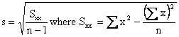
The two distributions shown in Figure 5.2
can, by a stretch of the imagination, be described as bell
shaped, but they are not symmetrical. Distributions like these,
having a "tail" on one side or the other, are said to be skewed;
if the tail is on the left we say that they are negatively
skewed and if the tail is on the right we say that they are
positively skewed. Distributions of incomes or wages are often
positively skewed because of the presence of some relatively
high values that are not offset by correspondingly low values.
|
Positive Skewed
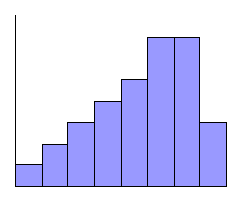
Negative Skewed |
Figure 5.2: Skewed distributions.
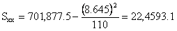
The
concepts of symmetry and skewness apply to any kind of data, not
only distributions. Of course, for a large set of data we may
just group the data and draw and study a histogram, but if that
is not enough, we can use anyone of several statistical measures
of skewness. A relatively easy one is based on the fact that
when there is perfect symmetry, the mean and the median will
coincide. When there is positive skewness and some of the high
values are not offset by correspondingly low values, as shown in
Figure 5.3, the mean will be greater than the median; when there
is a negative skewness and some of the low values are not offset
by correspondingly high values, the mean will be smaller than
the median.
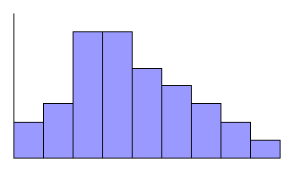
Figure 5.3: Mean and median of positively skewed distribution
This
relationship between the median and the mean can be used to
define a relatively simple measure of skewness, called the
Pearsonian coefficient of skewness. It is given by
|
Pearsonian coefficient of skewness |
 |
For
a perfectly symmetrical distribution, such the mean and the
median coincide and SK = 0. In general, values of the Pearsonian
coefficient of skewness must fall between -3 and 3, and it
should be noted that division by the standard deviation makes SK
independent of the scale of measurement.
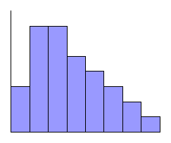
Example (6)
Calculate SK for the distribution of the waiting times
between eruptions of Old Faithful, using the results of Examples
3.21, 3.22, and 4.7, where we showed
 ,
and s = 14.35. ,
and s = 14.35.
Solution:
Substituting these values into the formula for SK, we get
Which shows that there is a definite, though modest, negative
skewness. This is also apparent from the histogram of the
distribution, shown originally and here again in Figure 5.4,
reproduced from the display screen of a TI-83 graphing
calculator.
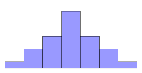
Figure 5.4: Histogram of distribution of waiting times between
eruptions of old faithful
When
a set of data is so small that we cannot meaningfully construct
a histogram, a good deal about its shape can be learned from a
box plot
(defined originally). Whereas the Pearsonian
coefficient is based on the difference between the mean and the
median, with a box plot we judge the symmetry or skewness of a
set of data on the basis of the position of the median relative
to the two quartiles, Q1 and Q3. In
particular, if the line at the median is at or near the center
of the box, this is an indication of the symmetry of the data;
if it is appreciably to the left of center, this is an
indication that the data are positively skewed; and if it is
appreciably to the right of center, this is an indication that
the data are negatively skewed. The relative length of the two
"whiskers," extending from the smallest value to QI
and from Q3 to the largest value, can also be used as
an indication of symmetry or skewness.
Example (7)
Following are the annual incomes of fifteen CPAs in thousands of
dollars: 88, 77, 70, SO, 74, 82, 85, 96, 76, 67, 80, 75, 73, 93,
and 72. Draw a box plot and use it to judge the symmetry or
skewness of the data.
Solution:
Arranging the data according to size, we get
|
|
67 |
70 |
72 |
73 |
74 |
75 |
76 |
77 |
|
|
80 |
80 |
82 |
85 |
88 |
93 |
96 |
|
It
can be seen that the smallest value is 67; the largest value is
96; the median is the eighth value from either side, which is
77; Q1 is the fourth value from the left, which is
73; and Q3 is the fourth value from the right, which
is 85. All this information is summarized by the MINITAB
printout of the box plot shown in Figure 5.5. As can be seen,
there is a strong indication that the data are positively
skewed. The line at the median is well to the left of the
center of the box and the "wisker" on the right is quite a bit
longer than the one on the left.

|
|
65 75
85 95
C2 |
Figure 5.5: Box plot of incomes of the CPAs.
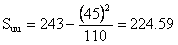
Besides the distributions we have discussed in this section,
two others sometimes met in practice are the reverse J-shaped
and U-shaped distributions shown in Figure 5.6. As can be
seen from this figure, the names of these distributions
literally describe their shapes. Examples of such
distribution may be found in real life situations.
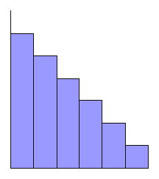 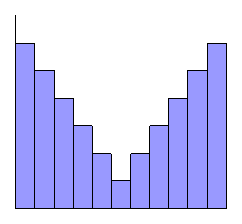
Figure 5.6: Reverse J-shaped and U-shaped
distributions |
|
|
|
|