6.1 Introduction

This objective of this chapter is to analyze the relationship among quantitative variables. Regression analysis is used to predict the value of one variable on the basis of other variables. This technique may be the most commonly used statistical procedure because, as you can easily appreciate, almost all companies and government institutions forecast variables such as product demand, interest rates, inflation rates, prices of raw materials, and labor costs by using it.

The technique involves developing a mathematical equation that describes the relationship between the variable to be forecast, which is called the dependent variable, and variables that the statistician believes are related to the dependent variable. The dependent variable is denoted y, while the related variables are called independent variables and are denoted x₁, x₂, …x_k (where k is the number of independent variables).

If we are interested only in determining whether a relationship exists, we employ correlation analysis. We have already introduced this technique. We presented the graphical method to describe the association between two quantitative variables - the scatter diagram. We introduced the coefficient of correlation and covariance.

Because regression analysis involves a number of new techniques and concepts. In this chapter, we present techniques that allow us to determine the relationship between only two variables.

Here are three examples of regression analysis.

Example (1)

The product manager in charge of a particular brand of children's breakfast cereal would like to predict the demand for the cereal during the next year. In order to use regression analysis, she and her staff list the following variables as likely to affect sales.

Price of the product

Number of children 5 to 12 years of age (the target market)

Price of competitor's products

Effectiveness of advertising (as measured by advertising exposure)

Annual sales this year

Annual sales in previous years

Example (2)

A gold speculator is considering a major purchase of gold bullion. He would like to forecast the price of gold two years from now (his planning horizon) using regression analysis. In preparation, he produces the following list of independent variables.

Interest rates

Inflation rate

Price of oil

Demand for gold jewelry

Demand for industrial and commercial gold

Dow Jones Industrial Average

Example (3)

A real estate agent wants to more accurately predict the selling price of houses. She believes that the following variables affect the price of a house.

Size of the house (number of square feet)

Number of bedrooms

Frontage of the lot

Condition

Location

In each of these examples, the primary motive for using regression analysis is forecasting. Nonetheless, analyzing the relationship among variables can also be quite useful in managerial decision making. For instance, in the first application, the product manager may want to know how price is related to product demand so that a decision about a prospective change in pricing can be made.

Another application comes from the field of finance. The capital asset pricing model analyzes the relationship between the returns of a particular stock and the behavior of a stock index. Its function is not to predict the stock's price but to assess the risk of the stock versus the risk of the stock market in general.

Regardless of why regression analysis is performed, the next step in the technique is to develop a mathematical equation or model that accurately describes the nature of the relationship that exists between the dependent variable and the independent variables. This stage – which is only a small part of the total process – is described in the next section. Only when we're satisfied with the model do we use it to estimate and forecast.

6.2 Model

The job of developing a mathematical equation can be quite complex, because we need to have some idea about the nature of the relationship between each of the independent variables and the dependent variable. For example, the gold speculator mentioned in Example 2 needs to know how interest rates affect the price of gold. If he proposes a linear relationship, that may imply that as interest rates rise (or fall), the price of gold will rise or fall. A quadratic relationship may suggest that the price of gold will increase over a certain range of interest rates but will decrease over a different range. Perhaps certain combinations of values of interest rates and other independent variables influence the price in one way, while other combinations change it in other ways. The number of different mathematical models that could be proposed is virtually infinite.

You might have encountered various models in previous courses. For instance, the following represent relationships in the natural sciences.

E = mc², where E = Energy, m = Mass, and c = Speed of light

F = ma, where F = Force, m = Mass, and a = Acceleration

S = at²/2, where S = Distance, t = Time, and a = Gravitational acceleration

In other business courses, you might have seen the following equations.

Profit = Revenue - Costs

Total cost = Fixed cost + (Variable cost X Number of units produced)

The above are all examples of deterministic models, so named because - except for small measurement errors - such equations allow us to determine the value of the dependent variable (on the left side of the equation) from the value of the independent variables. In many practical applications of interest to us, deterministic models are unrealistic. For example, is it reasonable to believe that we can determine the selling price of a house solely on the basis of its size? Unquestionably, the size of a house affects its price, but many other variables (some of which may not be measurable) also influence price. What must be included in most practical models is a method that represents the randomness that is part of a real-life process. Such a model is called probabilistic.

To create a probabilistic model, we start with a deterministic model that approximates the relationship we want to model. We then add a random term that measures the error of the deterministic component. Suppose that in Example 3 described above, the real estate agent knows that the cost of building a new house is about $75 per square foot and that most lots sell for, about $25,000. The approximate selling price would be

Y=25,000+75x

Where y = Selling price and x = Size of the house in Square feet. A house of 2,000 square feet would therefore be estimated to sell for

y =25,000 + 75(2,000) = 175,000 )

We know, however, that the selling price is not likely to be exactly $175,000. Prices may actually range from $100,000 to $250,000. In other words, the deterministic model is not really suitable. To represent this situation properly, we should use the probabilistic model.

Y = 25,000+75x + 

Where  (the Greek letter epsilon) represents the random term (also called the error variable) – the difference between the actual selling price and the estimated price based on the size of the house. The random term thus accounts for all the variables, measurable and immeasurable, that are not part of the model. The value of  will vary from one scale to the next, even if x remains constant. That is, houses of exactly the same size will sell for different prices because of differences in location, selling season, decorations, and other variables.

In the regression analysis, we will present only probabilistic models. Additionally, to simplify the presentation, all models will be linear. In this chapter, we restrict the number of independent variables to one. The model to be used in this chapter is called the first-order linear model – sometimes called the simple linear regression model.

First-Order Linear Model

where

            y= dependent variable

            x = independent variable

             = y-intercept

             = slope of the line (defined as the ratio rise/run or

change in y/change in x)

 = error variable

Figure 6.1 depicts the deterministic component of the model.

Figure 6.1: First-order linear model, deterministic component

The problem objective addressed by the model is to analyze the relationship between two variables, x and y, both of which must be quantitative. To define the relationship between x and y, we need to know the value of the coefficients of the linear model  and. However, these coefficients are population parameters, which are almost unknown. In the next section, we discuss how these parameters are estimated.

6.3 Least Squares Method

We estimate the parameters and  in a way similar to the methods used to estimate all the other parameters discussed in this notes. We draw a random sample from the populations of interest and calculate the sample statistics we need. Because and represent the coefficients of a straight line, their estimators are based on drawing a straight line through the sample data. To see how this is done, consider the following simple example.

Example (4)

Given the following six observations of variables x and y,-determine the straight line that fits these data.

Solution:

As a first step we graph the data, as shown in the figure. Recall that this graph is called a scatter diagram. The scatter diagram usually reveals whether or not a straight line model fits the data reasonably well. Evidently, in this case a linear model is justified. Our task is to draw the straight line that provides the best possible fit.

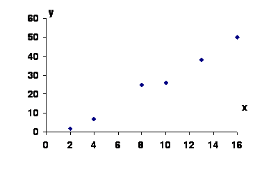
Scatter Diagram for Example

We can define what we mean by best in various ways. For example, we can draw the line that minimizes the sum of the differences between the line and the points. Because some of the differences will be positive (points above the line), and others will be negative (points below the line), a canceling effect might produce a straight line that does not fit the data at all. To eliminate the positive and negative differences, we will draw the line that minimizes the sum of squared differences. That is, we want to determine the line that minimizes.

Where y_i represents the observed value of y and  represents the value of y calculated from the equation of the line. That is,

The technique that produces this line is called the least squares method. The line itself is called the least squares line, or the regression line. The "hats" on the coefficients remind us that they are estimators of the parameters  and .

By using calculus, we can produce formulas for   and .Although we are sure that you are keenly interested in the calculus derivation of the formulas, we will not provide that, because we promised to keep the mathematics to a minimum. Instead, we offer the following, which were derived by calculus.

Calculation of  and .

where

and where

The formula for SS_x should look familiar; it is the numerator in the calculation of sample variance s². We introduced the SS notation; it stands for sum of squares. The statistic SS_x is the sum of squared differences between the observations of x and their mean. Strictly speaking, SS_xy is not a sum of squares.

The formula for SS_xy may be familiar; it is the numerator in the calculation for covariance and the coefficient of correlation.

Calculating the statistics manually in any realistic Example is extremely time consuming. Naturally, we recommend the use of statistical software to produce the statistics we need. However, it may be worthwhile to manually perform the calculations for several small-sample problems. Such efforts may provide you with insights into the working of regression analysis. To that end we provide shortcut formulas for the various statistics that are computed in this chapter.

Shortcut Formulas for SS_x and SS_xy

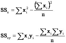
As you can see, to estimate the regression coefficients by hand, we need to determine the following summations.

Sum of x:

Sum of y:

Sum of x-squared:

Sum of x times y:

Returning to our Example we find

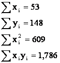
Using these summations in our shortcut formulas, we find

and

Finally, we calculate

and

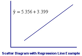
Thus, the least squares line is

The next figure describes the regression line. As you can see, the line fits the data quite well. We can measure how well by computing the value of the minimized sum of squared differences. The differences between the points and the line are called residuals, denoted r_i .   That is,

The residuals are the observed values of the error variable. Consequently, the minimized sum of squared differences is called the sum of squares for error denoted SSE.

Sum of Squares for Error

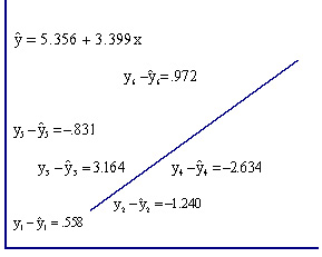
The calculation of SSE  this Example is shown in the next figure. Notice that we compute Yi by substituting Xi into the formula for the regression line. The residuals are the differences between the observed values and the computed values. The following Table describes the calculation of SSE.

Thus, SSE = 20.4332. No other straight line will produce a sum of squared errors as small as 20.4332. In that sense, the regression line fits the data best. The sum of squares for error is an important statistic because it is the basis for other statistics that assess how well the linear model fits the data.

Example (5)

We now apply the technique to a more practical problem.

Example (6)

Car dealers across North America use the "Red Book" to help them determine the value of used cars that their customers trade in when purchasing new cars. The book, which is published monthly, lists the trade-in values for all basic models of cars. It provides alternative values of each car model according to its condition and optional features. The values are determined on the basis of the average paid at recent used-car auctions. (These auctions are the source of supply for many used-car dealers.) However, the Red Book does not indicate the value determined by the odometer reading, despite the fact that a critical factor for used – car buyers is how far the car has been driven. To examine this issue, a used-car dealer randomly selected 100 three year of Ford Taurusses that were sold at auction during the past month. Each car was in top condition and equipped with automatic transmission, AM/FM cassette tape player, and air conditioning. The dealer recorded the price and the number of miles on the odometer. These data are summarized below. The dealer wants to find the regression line.

Solution:

Notice that the problem objective is to analyze the relationship between two quantitative variables. Because we want to know how the odometer reading affects selling price, we identify the former as the independent variable, which we used, and the latter as the dependent variable, which we label y.

Solution by Hand:

To determine the coefficient estimates, we must compute SS_x and SS_xy. They are

and

Using the sums of squares, we find the slope coefficient.

To determine the intercept, we need to find x and y. They are

and

Thus,

The sample regression line is

Interpreting The Coefficient

The coefficient  which means that for each additional mile on the odometer, the price decreases by an average of $0.0312 (3.12 cents).

The intercept is. Technically, the intercept is the point at which the regression line and the y-axis intersect. This means that when x = 0 (i.e., the car was not driven at all) the selling price is $6,533. We might be tempted to interpret this number as the price of cars that have not been driven. However, in this case, the intercept is probably meaningless. Because our sample did not include any cars with zero miles on the odometer we have no basis for interpreting. As a general rule, we cannot determine the value of y for a value of x that is far outside the range of the sample values of x. In this example, the smallest and largest values of x are 19,057 and 49,223, respectively. Because x = 0 is not in this interval we cannot safely interpret the value of 11 when x = o.

6.4 Assessing the Model

The least squares method produces the best straight line. However, there may in fact be no relationship or perhaps a nonlinear (e.g., quadratic) relationship between the two variables. If so, the use of a linear model is pointless. Consequently, it is important for us to assess how well the linear model fits the data. If the fit is poor, we should discard the linear model and seek another one. 

6.5 Using the Regression Equation

 Using the techniques in Section 5, we can assess how well the linear model fits the data. If the model fits satisfactorily, we can use it to forecast and estimate values of the dependent variable. To illustrate, suppose that in Example 2, the used car dealer wanted to predict the selling price of a three-year-old Ford Taurus with 40,000 miles on the odometer. Using the regression equation, with x = 40,000, we get

Thus, the dealer would predict that the car would sell for $5,285.

6.6 Coefficients of Correlation 

When we introduced the coefficient of correlation (also called the Pearson coefficient of correlation), we pointed out that it is used to measure the strength of association between two variables.