Chapter 3: ‎  Risk Assessment

Contents:

Having identified possible sources of risk to the project, we need to calculate their impact on the project. First we calculate the impact of individual risks, and then determine their combined impact.

3.1

The Impact of Risk

3.1 The Impact of Risk

The Impact of a risk factor depends on its likelihood of occurring and the consequence if it does occur:

   Impact of risk = (Likelihood of risk) * (Consequence of risk)

To illustrate this concept, consider the question of whether buildings in Aswan have earthquake protection. The answer is: very few or none have.

The consequence of an earthquake of force 8 on the Richter Scale would be severe loss of life, however the probability (likelihood) of such an earthquake is so small, virtually zero, that it is considered unnecessary to take any precautions in ordinary buildings.

But Aswan Reservoir and Aswan Dam do have earthquake protections.

The likelihood of an earthquake is the same but the consequences of that risk occurrence are unacceptably high income of the reservoir and the dam.

3.2

Risk Assessment of Several Risks Combined

The Top-Down Approach

The Bottom-Up Approach

Risk Assessment of Several Risks Combined

Case Study: It is a rare project that has only a single source of risk, so to determine the total impact of risk on a project the elements must be combined. If we include all possible sources of risk into the model, it will become impossibly complicated, so we limit our attention to the significant few, the 20 per cent that have 80 per cent of the impact. The work breakdown structure is a key tool in this integration of the risk. In practice, there are two approaches:

- A top-down approach, in which key risk factors are identified and assessed at a high level of work breakdown, and managed out of the project

- A bottom-up approach. in which risks are identified at a low level of work breakdown, and an appropriate contingency made to allow for the risk

3.2.1 The Top-Down Approach

The top-down approach can provide managers with checklist of potential risk factors based on previous experience and can help them to determine each risk's relative importance. Furthermore, by identifying the controlling relationships at a high level it enables project managers to find ways of eliminating the most severe risks from their projects.

Figure 3.1 is the top-level network for a simple project to build a warehouse where there are four packages of work, see Table 3.1. Assuming end-to-start dependencies only, the duration of the project is seven months. It might be possible to fast track the project by overlapping work packages. However let us assume that, that is impossible on the path A-C-D: it is not possible to buy the steel until the design is finished and because all the steel will arrive at once, erection cannot begin until the steel has arrived. It might be possible to start work on the site before the design is finished, but there is no need because the duration will be determined by the delivery of the steel.

Figure 3.1: Simple precedence network for constructing a warehouse

Table 3.1: Project to erect a warehouse

Now let us consider the risks. Let us assume that the project will start at the beginning of September, after the summer vacation. The risks are as follows:

1.      The design of the building may take more or less than three months. From previous experience, we may be able to say it will take two, three or four months with the following probabilities:

-          2 months: 25 per cent

-          3 months: 50 per cent

-          4 months: 25 per cent

Hence it may be finished as early as the end of October, or may stretch to the end of December.

2.      The site cannot he prepared if there is snow on the ground. Snow occurs in four months of the year with the following probabilities :

-          December: 25 per cent

-          January: 25 per cent

-           February: 50 per cent

-          March: 25 per cent

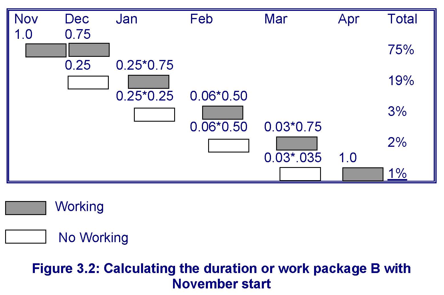
The duration of this work package is dependent on when it starts. If it starts in October, it will take only two months; if it starts in November, it will have the following range of durations, see Figure 3.2.

-          2 months: 75 per cent

-          3 months: 19 per cent

-          4 months: 3 per cent

-          5 months: 2 per cent

-          6 months: 1 per cent

There will be similar tables if the work were to start in December or January, but with the probabilities weighted towards the longer durations. In some circumstances, the preparation of the site will become critical. Now it may be worthwhile trying to fast track the design of the foundations. If the design could be completed by the end of September, we could eliminate this risk entirely. If it is finished by the end of October, there is a 75 per cent chance of the work being finished on time. If the start of this work is delayed to December, there is only a 50 per cent chance. The choice will depend on the cost of fast tracking the design of the foundations. There will be additional financial charges if this work is completed early, it is unlikely that the cost of the design will be greater per se, but there is a risk of re-work as described above in identifying risk. In the event, you may actually make the decision on the day depending on how the design of the steelwork is progressing, and on other factors below.

Figure 3.2: Calculating the duration or work package B with November start

1.      There may be two possible suppliers of steelwork: the more expensive one can deliver in one month or two months with equal probability; and the cheaper in two months or three months also with equal probability. The delivery time therefore has the following distribution:

                             -   1 month: 25 per cent

-          2 months: 50 per cent

-          3 months: 25 per cent

On the face of it, this appears the same as the design. However, the power of this top-down approach is you can decide what to do on the day when you know how long the design has taken and how you are progressing with the foundations. To understand this we need to address the fourth risk.

2.      This is that the steelwork cannot be erected if there are strong winds, and these occur with the following probability:

-          February: 25 per cent

-          March: 50 per cent

The duration of this work will also depend on when it starts as with preparing the site. However, what we can see is that if the design work finishes at the end of October then it will be better to use the more expensive supplier. There will then be a 50 percent chance that erection can begin in December and finish in January without any delay, or a 50 per cent chance that it will begin in January, in which case it will finish in February with a 75 per cent chance. This is of course dependent on the foundations being ready, and so if it looks as though the steelwork design will be completed early then it will be worthwhile fast tracking the foundations. On the other hand, if the design takes four months, it would be better to use the cheaper supplier and just plan to start erecting the steelwork in April saving on extra cost of the foundations and on having erection fitters standing idle.

This simple case shows that the top-down approach allows you to analyze the interrelationships between elements of risk, and management decisions based on that analysis and the actual out-turn. Following a top-down approach, you are able to develop additional detail in some areas. In the case above, for instance you could introduce a lower level of work breakdown to find out how to fast track the design of the foundations to reduce the risk. That requires the design to be broken into smaller packages of work subject to strict design parameters at the top level.

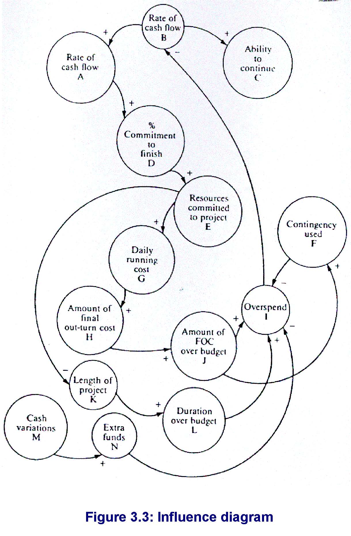
3.2.2 Influence Diagrams

Influence diagrams are tools - derived from a systems dynamics approach -that can assist a top-down analysis. They show how risks influence one another: some risks reinforce others (+), and some reduce others (-). Figure 3.3 is an example of an influence diagram. The power of the technique is to identify loops of influence. “Vicious cycles” have an even (or zero) number of negative influences, and “stable cycles” an odd number. In Figure 3.3 loop ADEKLIBA is vicious, and loop ADEGHJIBA is stable. In “vicious cycle” an externally imposed influence can be amplified indefinitely.

3.2.3 The Bottom-Up Approach

The bottom-up approach analyses risk at a low level. It can identify several critical paths, and calculate a range of outcomes for cost and duration to enable the project manager to allow appropriate contingency. However, it is essentially a negative approach to risk, as it assumes that risk elements are beyond the control of managers. It does nothing to help the manager to quantify or convey information for developing an appropriate management response to reducing or eliminating risk.

The approach develops a detailed project model at a low level of breakdown. Variable durations and / or costs are assigned to work element, as in the above example. However, at a low level it is not possible to calculate the various outcomes manually, as they were above. Instead, we perform a Monte Carlo analysis. The project model is analyzed many times: 100 to 10 000 is typical depending on the size of the model. Each time a random number is drawn for each parameter for which there is a range of values, and a value selected accordingly. This makes the simplifying assumption that the risk elements are unrelated which may not be the case, see Figure 3.3. The cost and duration are then calculated using those values and a range of possible outcomes calculated for the project. Effectively, the project is sampled however many times the analysis is performed. The results of the Monte Carlo analysis are presented as a probability distribution for time cost or both. 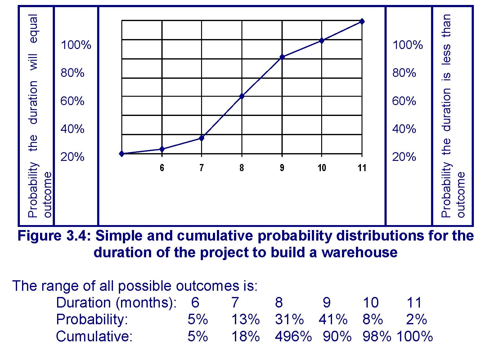This may be a simple or cumulative distribution. Figure 3.4 shows both distributions for the duration of the warehouse project, assuming the logic given in Table 3.1. For this simple case, the critical path may go through either A-B-D or A-C-D, and the duration can be anything from 6 to II months. The likelihood that either or both of the routes will be the critical path is:

Figure 3.3: Influence diagram

 Figure 3.4: Simple and cumulative probability distributions for the duration of the project to build a warehouse

The range of all possible outcomes is:

Duration (months):    6         7          8          9         10        11

Probability:                 5%      13%    31%    41%    8%      2%

Cumulative:                5%      18%    496%  90%   98% 100%

With a project this small, it is just possible to calculate these numbers by hand. With anything larger, the figures have to be determined using a Monte Carlo analysis. From this we see that the median outcome is eight months (half the time and the duration will be this or less) and that 90 percent of the time the duration will be less than nine months. The most likely duration (the mode) is nine months. If nine month duration is acceptable, we may accept these figures. If not, we would need to shorten the project. The critical path figures show that the most useful effort may be put into shortening A-B-D and that may suggest fast tracking the design of the foundations. However, from this we do not see the effect of the two suppliers. That can only be analyzed by the top- down approach.

3.3

Accounting for Increased Costs or Reduced Revenues

3.3 Accounting for Increased Costs or Reduced Revenues

Monte Carlo analysts can also be applied to the costs and revenues of a project, to produce a range of likely returns. However, with the costs and revenues, the risk can be accounted for directly by allowing a contingency.

3.4

Communicating the Risk Analysis

3.4 Communicating the Risk Analysis

The ultimate purpose of the risk model is to communicate the analysis to all the parties involved with the project:

-         to the owners for them to assess its value,

-         to the champions, so they can give their support and commitment to the project,

-         to the project managers so that they can develop their project strategies and perform what-if analyses,

-         to the integrators, to enable them to manage the risks during implementation,

-         to people joining the project at a later time so they know what assumptions have been made, and

-         to the users so that they know the commitments they are making.